Learning by Gradient Descent: Stochastic Approximation

Learning with Machines on large multidimensional datasets can be computationally intensive especially if significant batches of data samples are necessary or used for each learning step - as in batch gradient descent for perceptron training. However, if at each learning step, the learning is not differentiable, we end up with an iteration of next to similar steps on the gradient slope which do not significantly say a lot about the learning machine.

Let’s first understand what Gradient descent is, variations of it and how stochastic approximation can come into play. Using a simple explanation given in the Deep Learning Book(Ian Goodfellow et al);

Consider an objective function \(f(x)\) that we want to optimize i.e. minimize or maximise it by altering x. 

We obtain its derivative \(f^1(x)\) which gives the slope of \(f(x)\) at point x, thus we can scale a change in input to obtain a corresponding change in output. For examples \(f(x +\in) \sim f(x) + \in f^1(x)\). Therefore, to minimize the function \(f(x)\), we can move small steps in the opposite direction of the derivative \(f^1(x)\). That is basically gradient descent.

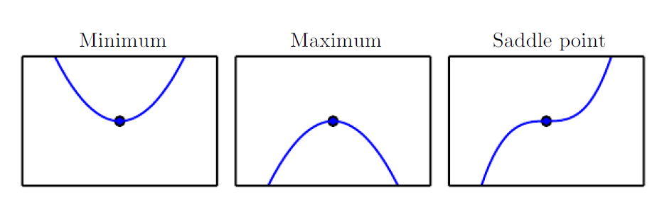
The objective function and its derivative values represent crucial parts of the gradient learning ; \(f^1(x) = 0 \), which are referred to as critical or stationary points which provide no information about direction of gradient and these points fall within the following categories;

• Local minima- refers to a point lower than all neighboring points
• Local Maxima - refers to a point higher than all neighboring points
• Saddle points - Neither a maxima or minima
• Global Minima - is the lowest value of f(x) throughout the input space and it is highly possible for a local minima not to be globally optimum

Beyond and/or above the local maxima and minima it is not possible to increase and/or decrease the value of \(f(x)\).

Gradient Update rule

The general Gradient Update rule can be defined as follows;

In this case, we consider perceptron learning of weights(Haykin has a great explanation) over \(t\) learning steps and \(E\) is the cost function. Therefore the next weight \(w_{t+1}\) can be estimated by the current \(w_t\) minus a product of the learning rate \(\eta\) and a derivative of the cost function \(E\) w.r.t the weight.

The negative gradient gives the direction of the steepest descent in E.

Further we will explore the types of gradient descent; Batch which was mentioned earlier and online learning which processes each observation, one at a time, updating the gradient after learning step. Online learning has several advantages over the Batch learning i.e no need to store complete dataset, easy adaptability in cases of changing data and many more.

Learning gradient descent with stochastic approximation is basically online learning but the singular examples are selected randomly with equal probability at each learning update for \(tmax \cdot P\) learning steps(P is the number of observations in the dataset). Therefore the true gradient of the cost function \(E\) is approximated by a single example.

Below are my Matlab code samples that can be refactored into any programming langauge.

sgd.m

function [w1,w2,E_cost,test_error] = sgd(xi,tau, P,Q,eta,tmax)
% Input
% eta - learning rate
% P - number of training sets
% Q -number of test sets
% xi - input vectors 50 x 5000 vector
% tau - corresponding labels
% eta - learning rate
% tmax - number of learning steps

    % w1 and w2 - N dim vectors of adpative input to hidden networks
    %Initialize the weights as independent random vectors with |w1|^2 = 1 and
    %|w2|^2 = 1.
    N = length(xi(:,1));
    w1 = rand(N,1);
    w1 = w1/norm(w1);
    w2 = rand(N,1);
    w2 = w2/norm(w2);

    E_cost = zeros(tmax,1); % stores the cost function E(t)
    test_error = zeros (tmax,1); % E_test(t)
    % Stochastic gradient descent procedure
    for i = 1: tmax
        for example = 1:P
            % In each learning step, select one of the P example randomly
            index = randi(P); % equal probability
            %gradient with respect to random input
            xi_v = xi(:,index);
            tau_v = tau(index);
            t1 = dot(w1,xi_v);
            t2 = dot(w2,xi_v);
            sigma = tanh(t1) +tanh(t2);
                        
            delta1 = (sigma - tau_v)* (1-tanh(t1)^2) * xi_v; %gradient with w.r.t w1
            delta2 = (sigma - tau_v)* (1-tanh(t2)^2) * xi_v; %gradient  with w.r.t w2

            w1 = w1 - (eta*delta1);
            w2 = w2 - (eta*delta2); 
        end
        
        %Compute E and Etest after P single randomized steps, not after each individual update
        [E,E_test] = cost(w1,w2,xi,tau,P,Q);
        
        E_cost(i) = E;
        test_error(i) = E_test;

    end
end

cost.m

function [E,E_test] = cost(w1,w2,xi,tau,P,Q)
%Compute E and Etest after P single randomized steps, not after each individual update. It is
%recommended to define a (matlab) function which calculates E and Etest with w1, w2 and the
%corresponding data set (inputs and labels) as arguments.

% input
% P - number of training sets
% Q - number of test sets - Q -100 or larger
% w1 and w2 - weight vectors
% xi - input vector 50 X 5000
% tau - correpsonding continuos labels

% E - costfunction
%E_test - test/generalization error

% cost function
ee_sum =0;
for mu= 1:P
    xi_mu = xi(:,mu);
    tau_mu = tau(mu);% label of correspondin xi_mu
    t1 = dot(w1,xi_mu);
    t2 = dot(w2,xi_mu);
    sigma = tanh(t1) +tanh(t2);
    ee = (sigma - tau_mu)^2;
    ee_sum = ee_sum + ee;
end
E = ee_sum /(2*P);
% test/generalization error
ee_test =0;
for mu_test= (P+1): P+Q
    xi_mutest = xi(:,mu_test);
    tau_mutest= tau(mu_test);% label of correspondin xi_mu
    t11 = dot(w1,xi_mutest);
    t22 = dot(w2,xi_mutest);
    sigma_test = tanh(t11) +tanh(t22);
    ee_t = (sigma_test - tau_mutest)^2;
    
    ee_test = ee_test+ ee_t;
end
E_test = ee_test / (2*Q);
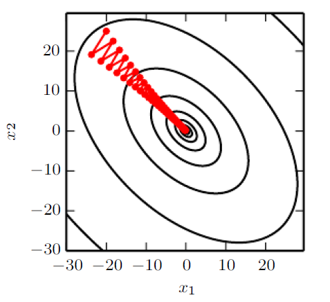
end

The cost function and generalisation error values can be calculated after \(P\) randomised steps to monitor the learning performance. As seen below, we can see plateau states in the cost function after certain learning steps. At these points there isn’t much learning happening therefore the generalisation error will significantly increase. This behavior can also explain poor generalisation and overfitting at the plateau states.

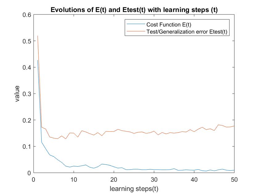
Figure shows plateau states from Stochastic Gradient descent

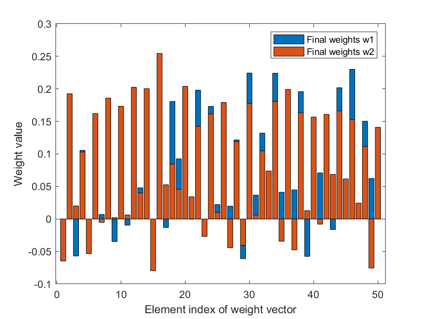
Figure shows final weights from Stochastic Gradient descent. The weights signify the importance of the features

Further reading/ Reference material

-Deep learning by Ian Goodfellow, Yoshua Bengio, Aaron C. Courville

-The Elements of statistical learning by Jerome H. Friedman, Robert Tibshirani, and Trevor Hastie

-Neural networks and learning machines by Simon S. Haykin